For this case, the NACA 0012 grids(1) and results from John Vassberg's and Antony Jameson's grid convergence study(2) were used to verify AT CFD and to study the grid convergence of AT CFD. I would like to thank John Vassberg for allowing me to use the grids. The values presented in this documentation for FLO82, OVERFLOW, and CFL3D came from AIAA.2009-4114(2).
Introduction
The approach taken by J. Vassberg and A. Jameson in their study was to create a set of extremely high quality 0-meshes about a NACA 0012 grid. The finest grid contains 4096x4096 cells. The remaining grids are created by removing every other line in each direction from the previous finer grid. This results in the following grid family; 4096x4096, 2048x2048, 1024x1024, 512x512, 256x256, 128x128, 64x64, 32x32. Euler results are then obtained over the set of grids using three CFD codes (FLO82, OVERFLOW, and CFL3D), and the grid convergences for lift, drag, and pitching moment are observed. The residuals for each run are converged to machine zero using 64 bit computations.
For the example presented here, two angles of attack (0.0 and 1.25) at two Mach numbers (0.5 and 0.8) were tested with AT CFD. A couple of far field and surface boundary conditions were also tested. At the far field a free stream and a characteristic boundary condition were used. At the surface a momentum boundary condition and a first order extrapolation condition were used.
In an effort to compare the AT CFD results to OVERFLOW, AT CFD was run in central finite differencing mode and an attempt was made to implement OVERFLOW's default settings in AT CFD. The dissipative scheme implemented in AT CFD already matched OVERFLOW's default dissipative scheme. The 2nd order dissipation value was set to 2.0(3) and the 4th order dissipation value was set to 0.04(3). In addition, the speed of sound in the spectral radius was replaced by |V|/M∞(3). It should be noted that access to OVERFLOW's source code did not exist nor were individuals knowledgeable about the internal workings of OVERFLOW contacted. Furthermore, it was assumed that the default settings were used by J. Vassberg and A. Jameson for the OVERFLOW runs. The authors were not contacted on this issue. Therefore, a rigorous effort to ensure that AT CFD matched OVERFLOW was not made.
In addition to determining the force and moment coefficients for the various AT CFD cases, the CFL value for maximum residual convergence rate was determined. The solutions were converged using local time stepping. The methodology consisted of making an educated guess for the initial run and then incrementing the CFL value till the maximum residual convergence rate was found. The CFL values for the 32x32 and 64x64 grids were incremented by 1.0. The CFL values for the remaining finer grids were incremented by 2.0. The CFL number is only presented for the AT CFD runs since the values are not given for the FLO82, OVERFLOW, and CFL3D results.
The use of the force and moment coefficients for the determination of the grid convergence shows an overall picture of how the solution converges with respect to grid size. To further illustrate the details of the rate of grid convergence, 2D plots and contour plots for the convergence of the pressures are presented.
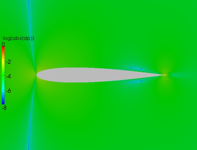
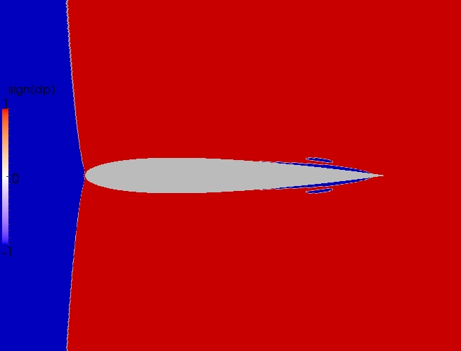
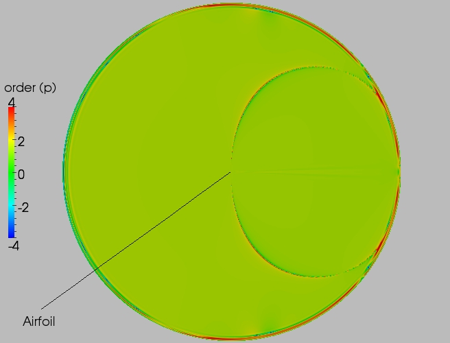
To help understand the grid convergence of AT CFD better, two sets of contour plots applied to pressure are shown for each converged solution. One set is focused on the airfoil and the other set is focused on the entire grid. Each set contains three plots. The first plot, called order(p), is the grid convergence order for pressure and is equal to log2(abs((pfine-pmedium)/(pmedium-pcoarse))). The pfine value is the pressure on the current grid, pmedium is the pressure on the next coarser from pfine, and pcoarse is the next coarser from pmedium. To calculate order(p), only the point locations from the coarse grid are used so the points from the three grids overlay. The second plot, called rate(p), is the grid convergence rate for pressure and is equal to log10(abs(pfine-pmedium)). The third plot, called sign(dp), is the grid convergence direction for pressure and is equal to sign(pfine-pmedium).
It is important to note that the rate of convergence of pressure is dependent both on the non linearity of the pressure equation and the rate of convergence for the state variables (ρ, ρu, ρv, ρw, and ρe0). Once the number of grid cells increases to the point where the rate of change of the pressure becomes a linear function of the rate of change of the state variables and the order of convergence of the state variables become independent of the number of grid cells, then the order of convergence of pressure, and thus loads, becomes independent of the number of grid cells.
In the end, it is difficult, for me, to say what the order of convergence for the integrated loads should be based on the fact that the Euler equations used are second order accurate. The most I'm willing to say is that the solution within a region somewhere in the field will converge at second order accuracy. However, the areas around that region may converge at a lower or higher order since the influence of that region may be diminishing or increasing non linearly. I don't think one should expect that the entire flow field converges uniformly at a constant order.
Example Case Examination
To help describe the data set for this overall example, one test case will be chosen and examined. The test case chosen is for Mach=0.5 and α=0.0. The boundary conditions for the test case are free stream for the outer and momentum for the surface. The Mach number of 0.5 was chosen since the flow does not contain a shock. The angle of attack of zero was chosen so that the runs from the various codes are equal in regards to not having a point vortex. The momentum boundary condition was chosen since it matches the FLO82, OVERFLOW, and CFL3D runs, it is higher order than extrapolation, it demonstrates high order grid convergence for the drag coefficient at moderate grid sizes, and it demonstrates a change in grid convergence rate at the finer grids. The free stream boundary condition was chosen for the outer boundary to demonstrate how the free stream boundary condition affects the grid convergence of the solution at the outer boundary. The selection of free stream or characteristic boundary condition at the outer boundary has minimal effect of the solution on the surface as demonstrated in the results section below. Furthermore, lagging the characteristic boundary condition is the limiting factor for the CFL value for maximum residual convergence. However, the free stream boundary condition, since it is constant, does not limit the CFL value for maximum residual convergence. It should be noted that, in general, the selection of a characteristic boundary condition for the outer boundary is appropriate and the selection of a free stream condition in this case is for demonstration purposes only.
To start things off, plotted below is the log base two of the CFL value for maximum residual convergence versus the log base two of the grid size.
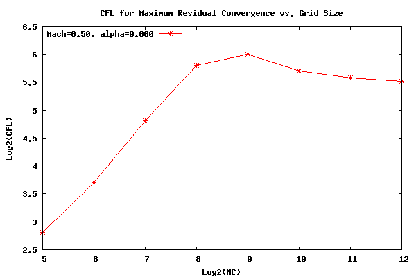
From the plot above it can be seen that the CFL for maximum residual convergence is close to scaling linearly with grid size for grids up to 256x256. In fact, the CFL number doubles with a doubling in the grid size. Past this point the CFL for maximum residual convergence decouples from the grid and converges to a constant as the grid size continues to increase. However, even at 4096x4096 the CFL for maximum residual convergence has not completely decoupled from the grid and it may take one or two more grid doublings to reach this point. Unfortunately, the workstation resources available have been maxed out with the 4096x4096 grid size. Since the CFL number has almost reached a constant, doubling the finest grid would require four times more memory and eight times more cpu time.
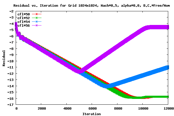
As an example of the residual convergence, the following plot shows the residual vs. iteration for four CFL values for the grid size of 1024x1024. From the graph it can be seen that the CFL value of 52 converges the fastest and that CFL values of 54 and 56 do not converge.
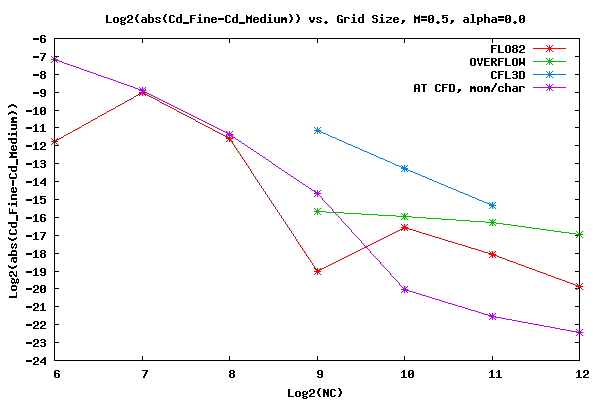
The following plot shows the grid convergence of Cd at Mach 0.50 and α 0.0 for AT CFD, FLO82, OVERFLOW, and CFL3D.
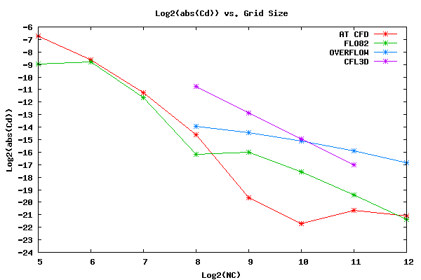
From the figure above it can be seen that the trend of grid convergence for Cd for AT CFD changes as the grid size increases. Ideally it would be beneficial to understand the convergence behavior past the finest grid. It should be noted that the first three Cd values for FLO82 are positive and the last five values for FLO82 are negative. It can be seen from the plot above that OVERFLOW converges at a slower rate than the other three codes. The reason for this is unknown. It is believed that there is little difference between OVERFLOW and AT CFD in regards to the right hand side of the implicit solution methodology. However, how OVERFLOW implements the momentum boundary condition is unknown.
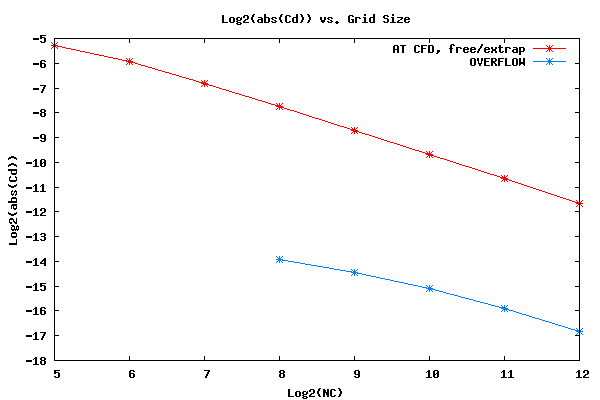
As a side note, the rate of convergence of OVERFLOW appears to be qualitatively similar to the rate of convergence when using an extrapolated boundary condition for AT CFD. The following plot compares the convergence of Cd for OVERFLOW to the convergence of Cd for AT CFD when the AT CFD surface boundary condition is set to extrapolate.
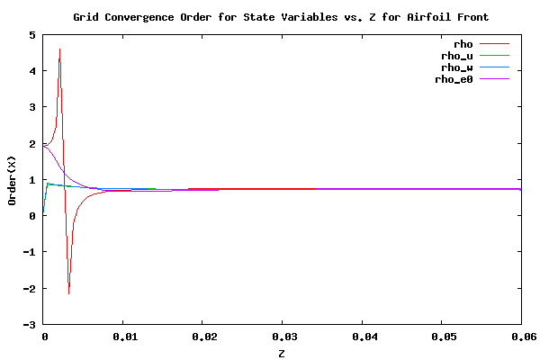
Switching back to the main discussion, the following plot shows the grid convergence order of pressure (p) vs. the airfoil height for the front facing airfoil surface. The grid convergence order of p is equal to log2(abs(pfine-pmedium)/(pmedium-pcoarse))). Only surface points which exist in all three of the fine, medium, and coarse grids were chosen. The pfine value is the pressure on the current grid, pmedium is the pressure on the next coarser grid from pfine, and pcoarse is the next coarser grid from pmedium. The plot below shows the order of p grid convergence for four grid sizes.
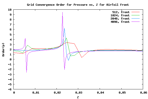
As can be seen from the plot above, the order of p for the four grids are similar and seem to be converging asymptotically to a curve. The spikes are a result of sign changes in the delta p from one grid to another. From a z value of 0.0 to about 0.005 the delta p is positive. From a z value of 0.005 to about 0.0225 the delta p is negative. From a z value of 0.0225 to 0.06 the delta p is positive.
The plot below shows the grid convergence rate of pressure (p) base two vs. the airfoil height for the front facing airfoil surface. The grid convergence rate of p base 2 is equal to log2(abs(pfine-pmedium)).
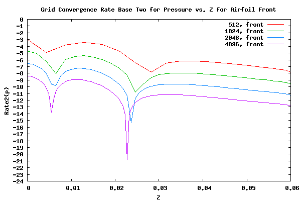
In the plot above, the difference between two curves represents the order of convergence. In general it appears that the curves have settled down to a characteristic shape and the overall order of convergence can be eyeballed as a value between 1.5 and 2.0. It can be seen that the pressure at the leading edge is converging at a faster rate than the point of maximum airfoil thickness. The order of convergence at the leading edge is just slightly higher than that at the point of maximum thickness.
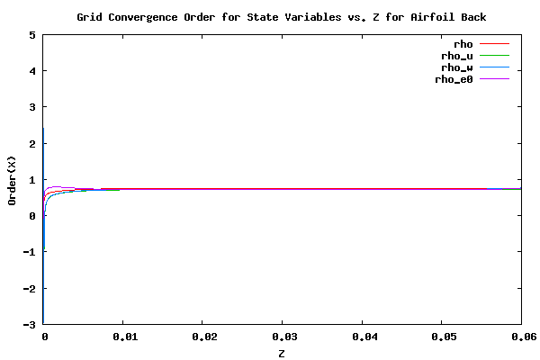
The following plot shows the grid convergence order of pressure vs. the airfoil height for the back facing airfoil surface.
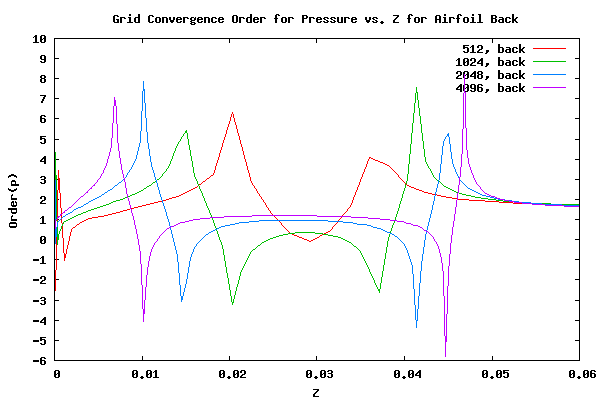
As can be seen from the plot above, more is occurring on the back side than the front side in regards to order of convergence. It will probably take at least two more grid refinements to establish the order of convergence of pressure and thus the convergence of the overall loads. Again, the spikes are a result of changes in the direction of convergence.
The plot below shows the grid convergence rate of pressure (p) base two vs. the airfoil height for the back facing airfoil surface.
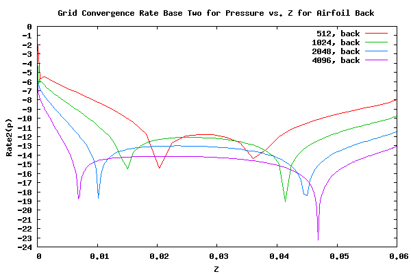
From the plot above it can be seen that a curve shape has yet to be settled upon and the order of convergence is not yet consistent between the curves. Again, it seems it will take at least two grid refinements to establish the characteristics. From the plot it can be seen that the order of convergence at the maximum airfoil thickness is faster than that halfway down the backside. It can also be seen that the rate of convergence halfway down the backside is accelerating. It is assumed that eventually the order of convergence halfway down the backside will match the order of convergence at the maximum thickness. It seems the order of convergence at the trailing edge is noticeably less than other areas. However this may be due to the fact that the point at which the sign for the rate of convergence changes has not been settled upon. Once that point is established the order of convergence may be more consistent with other areas of the backside.
As was noted above, the pressure is a function of the five state variables, ρ, ρu, ρv, ρw, and ρe0. To understand the grid convergence better it is necessary to examine how these variables converge. To examine this the following plots show the order of convergence of the state variables for the front and back sides of the finest grid, 4096x4096.
As can be seen from the plots above the order of convergence of the state variables are mostly smooth and constant. For the majority of the airfoil, the five state values have an order of convergence of about 0.75. However, as the leading edge of the airfoil is approached, the order of convergence of ρ and ρe0 approach 2.0. It should be noted that the difference in order of convergence between the various state variables are small of most of the airfoil. However, the difference, even though small, is an important factor in establishing the rate of convergence of the pressure. The difference is the reason the pressure converges at a significantly higher order than the state variables.
As was noted above, the order of convergence for ρ and ρe0 deviate from the order of convergence of the other state variables. This will be investigated further in the following plot. In the following plot the order of convergence for ρ and ρe0 for the front facing surface of the 4096x4096 and 2049x2048 grids are plotted together.
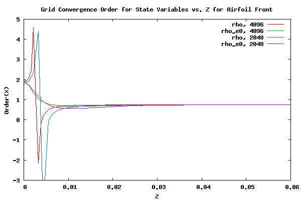
From the plot above it can be seen that the leading edge region over which the order of convergence changes is reducing in size as the number of grid points increases. It is hypothesized that as the number of grid points continues to increase the order of convergence curves will continue to flatten.
To get a better idea of the order of convergence in the field, the following contour plot shows the order of convergence of the pressure within the region of the airfoil.
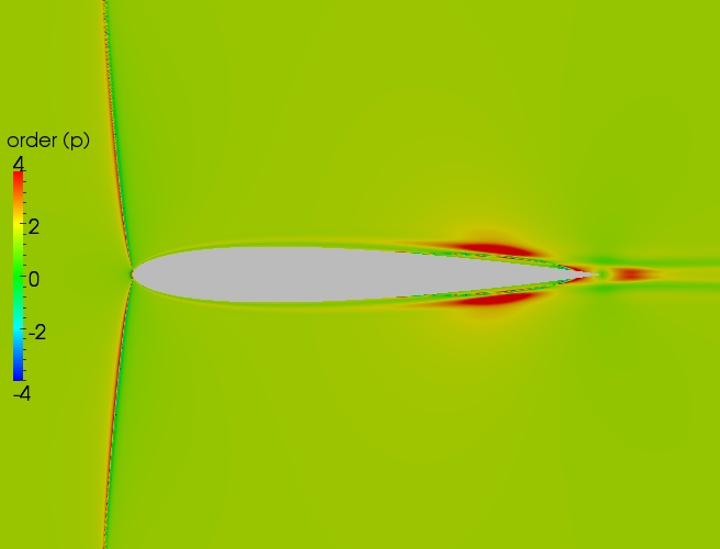
From the contour plot above it can bee seen that a band of 2nd order convergence exists off the surface of the airfoil. The band of higher than 2nd order convergence at the leading edge of the airfoil and off the top and bottom of the backward facing surface is due to a sign change. The reason for the higher than 2nd order convergence at, and aft, of the trailing edge is unknown. However, it is hypothesized that the reason is due to significant changes in that region due to changes in grid size. From investigating the order of convergence at the aft region for the 2048x2048 grid, it appears that the region is decreasing in size.
The plot below shows the rate of convergence for the pressure. Note that the plot below is log base ten of the change in pressure rather than the log base two.
The plot below shows the sign for the rate of change of the pressure. The sign change at the leading edge, as seen in the 2D plots above, can not be seen in the figure below since the sign change occurs only on the surface layer of grid points.
Finally, the plot below shows the order of convergence of the pressure for the entire grid. The airfoil is too small to be seen. The ring around the outer boundary is due to the free stream boundary condition. The ring does not exists with the characteristic boundary condition.
Informational Tidbits
Summarized below are informational tidbits related to this example.
| 1) | Due to bugs which were found and fixed during the analysis, the central finite differencing mode for AT CFD has become the only choice. Hopefully the finite volume mode will be fixed in the future. |
| 2) | Overall, the grid convergence trends compare somewhat with FLO82. However, there is a noticeable difference when compared to OVERFLOW. I suspect the momentum boundary condition for AT CFD is implemented different than OVERFLOW. |
| 3) | A point vortex on the farfield boundary condition was not used for AT CFD, thus differences between AT CFD and FLO82 exist at α=1.25. |
| 4) | Even with the finest grid, the grid convergence for AT CFD has reached the point where the order of the grid convergence can be determined. The solution around the airfoil is still changing qualitatively at the finest grid level, and the CFL value for maximum residual convergence has not reached an asymptotic value with respect to grid size. I suspect that once the CFL value has reached an asymptotic value then the solution will be qualitatively constant with respect to grid size. |
| 5) | The best choice of boundary conditions for this case in regards to accuracy is momentum for the surface and characteristic for the far field. |
| 6) | The solution methodology for AT CFD is such that the boundary values are lagged during an iteration. During an iteration, when solving for the flow variables in the interior, the boundary values are held constant. After the flow variables are updated the boundary conditions are enforced. The choice of boundary conditions affects the CFL value for maximum residual convergence. Using extrapolation for the surface and free stream for the far field resulted in the fastest residual convergence. Using characteristic for the far field resulted in the slowest residual convergence. |
| 7) | For AT CFD, the derivatives for the dissipation scheme's pressure switch and spectral radius are not included in the LHS. This effects the CFL value which can be used for maximum residual convergence when a shock exists. It appears that as the grid size increases the CFL value for maximum residual convergence, when a shock exists, drops dramatically. Reducing the 2nd order dissipation value negates this effect. |
Timing
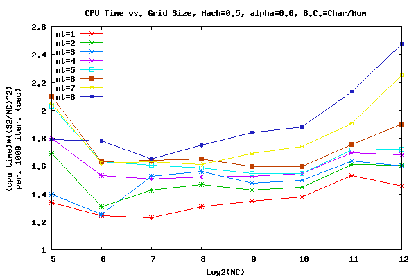
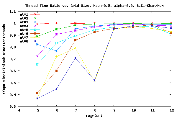
The following plot shows the total CPU time vs. grids size for the M=0.5 α=0.0 case. The total CPU time was normalized by a ratio of the grid size for better comparisons. The runs are for 1000 iterations and neglect IO. Runs from 1 to 8 threads were done. The number of threads (nt) is represented by a curve. It is important to note that total CPU time is plotted and not elapsed wall clock time. Therefore, in general, when the number of threads or the grid size is increased the total CPU time increases due to memory bandwidth bottle necks. The results at the smallest grid size should probably be neglected due to process scheduling uncertainties. The runs were done with an Intel Xeon DP Quad Core X5472 3.0Ghz 1600Mhz FSB processors and 8gb of 800MHz Fully Buffered DDR2 memory.
Results
Shown in the tables and plots below are all the results for this example. To view the order, rate, and sign contour plots of pressure convergence, select the CFL number in a table associated with the AT CFD run.
The figure below shows the log base two of the convergence rate of Cd for Mach=0.5 and α=0.00. As can be seen from the plot, FLO82, CFL3D, and AT CFD all have qualitatively the same convergence rate slope. The convergence rate slope for OVERFLOW appears to be different.
Shown below is the Cd data for M=0.5 and α=0.00. The AT CFD boundary condition is momentum and the surface boundary and characteristic at the far field boundary condition.
| NC | NC2 | FLO82-HCUSP | OVERFLOW-Central | AT CFD | CFL (AT CFD) |
| 32 | 1,024 | +0.001979418 | +0.009383374 | 9 | |
| 64 | 4,096 | +0.002270216 | +0.002524662 | 15 | |
| 128 | 16,384 | +0.000307646 | +0.000410972 | 32 | |
| 256 | 65,536 | -0.000013299 | +0.000063743 | +0.000039451 | 40 |
| 512 | 262,144 | -0.000015191 | +0.000044712 | +0.000001228 | 38 |
| 1,024 | 1,048,576 | -0.000005076 | +0.000028691 | +0.000000293 | 38 |
| 2,048 | 4,194,304 | -0.000001404 | +0.000016232 | +0.000000620 | 38 |
| 4,096 | 16,777,216 | -0.000000365 | +0.000008512 | +0.000000441 | 36 |
| ∞ | +0.000000045 | -0.000004058 | |||
Shown below is the Cd comparision for M=0.5 and α=0.00 for different AT CFD boundary conditions
| NC | cd (Char/Mom) | CFL (Char/Mom) | cd (Char/Ext) | CFL (Char/Ext) | cd (Free/Mom) | CFL (Free/Mom) | cd (Free/Ext) | CFL (Free/Ext) |
| 32 | +9.383374e-03 | 9 | +2.599680e-02 | 10 | +9.383527e-03 | 7 | +2.599629e-02 | 8 |
| 64 | +2.524662e-03 | 15 | +1.647651e-02 | 16 | +2.524687e-03 | 13 | +1.647647e-02 | 14 |
| 128 | +4.109717e-04 | 32 | +8.934423e-03 | 32 | +4.109747e-04 | 28 | +8.934425e-03 | 30 |
| 256 | +3.945072e-05 | 40 | +4.650430e-03 | 40 | +3.945138e-05 | 56 | +4.650431e-03 | 56 |
| 512 | +1.228482e-06 | 38 | +2.392124e-03 | 38 | +1.228749e-06 | 64 | +2.392124e-03 | 92 |
| 1,024 | +2.932144e-07 | 38 | +1.220307e-03 | 38 | +2.933506e-07 | 52 | +1.220307e-03 | 112 |
| 2,048 | +6.201276e-07 | 38 | +6.180074e-04 | 38 | +6.202163e-07 | 48 | +6.180074e-04 | 84 |
| 4,096 | +4.412920e-07 | 36 | +3.113151e-04 | 36 | +4.413639e-07 | 46 | +3.113151e-04 | 80 |
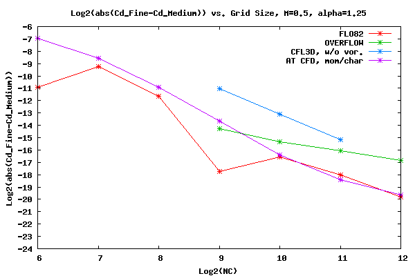
The figure below shows the log base two of the convergence rate of Cd for Mach=0.5 and α=1.25. As can be seen from the plot, FLO82, CFL3D, and AT CFD all have qualitatively the same convergence rate slope. The convergence rate slope for OVERFLOW appears to be different.
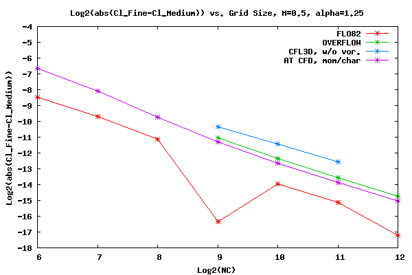
The figure below shows the log base two of the convergence rate of Cl for Mach=0.5 and α=1.25. As can be seen from the plot, FLO82, OVERFLOW, CFL3D, and AT CFD all have qualitatively the same convergence rate slope, except at the finest grid where FLO82 seems to have accelerated.
Shown below is the Cd data for M=0.5 and α=1.25. The AT CFD boundary condition is momentum and the surface boundary and characteristic at the far field boundary condition.
| NC | NC2 | FLO82-HCUSP | OVERFLOW-Central | AT CFD | CFL (AT CFD) |
| 32 | 1,024 | +0.002482085 | +0.011249519 | 8 | |
| 64 | 4,096 | +0.001974608 | +0.003226151 | 14 | |
| 128 | 16,384 | +0.000298397 | +0.000630306 | 32 | |
| 256 | 65,536 | -0.000011045 | +0.000118671 | +0.000106645 | 40 |
| 512 | 262,144 | -0.000015534 | +0.000068207 | +0.000029039 | 38 |
| 1,024 | 1,048,576 | -0.000005301 | +0.000044071 | +0.000017483 | 38 |
| 2,048 | 4,194,304 | -0.000001481 | +0.000029311 | +0.000014608 | 38 |
| 4,096 | 16,777,216 | -0.000000388 | +0.000020951 | +0.000013373 | 36 |
| ∞ | +0.000000050 | +0.000010030 | |||
Shown below is the Cl data for M=0.5 and α=1.25.
| NC | FLO82-HCUSP | OVERFLOW-Central | AT CFD |
| 32 | +0.181639135 | +0.1644426 | |
| 64 | +0.178822451 | +0.1742650 | |
| 128 | +0.180014345 | +0.1779383 | |
| 256 | +0.180458183 | +0.178960502 | +0.1791035 |
| 512 | +0.180446183 | +0.179435775 | +0.1795013 |
| 1,024 | +0.180382615 | +0.179627329 | +0.1796561 |
| 2,048 | +0.180354386 | +0.179710209 | +0.1797228 |
| 4,096 | +0.180347832 | +0.179747254 | +0.1797527 |
| ∞ | +0.180345850 | +0.179777193 | |
Shown below is the Cm data for M=0.5 and α=1.25.
| NC | FLO82-HCUSP | OVERFLOW-Central | AT CFD |
| 32 | -0.002926241 | -0.003741454 | |
| 64 | -0.002487849 | -0.002356471 | |
| 128 | -0.002294411 | -0.002168016 | |
| 256 | -0.002301404 | -0.002124907 | -0.002198558 |
| 512 | -0.002290609 | -0.002191480 | -0.002227430 |
| 1,024 | -0.002276577 | -0.002226157 | -0.002243920 |
| 2,048 | -0.002270586 | -0.002243944 | -0.002252870 |
| 4,096 | -0.002269217 | -0.002253042 | -0.002257534 |
| ∞ | -0.002268812 | -0.002262569 | |
Shown below is the Cd comparision for M=0.5 and α=1.25 for different AT CFD boundary conditions
| NC | cd (Char/Mom) | CFL (Char/Mom) | cd (Char/Ext) | CFL (Char/Ext) | cd (Free/Mom) | CFL (Free/Mom) | cd (Free/Ext) | CFL (Free/Ext) |
| 32 | +1.124951E-02 | 8 | +2.803419E-02 | 9 | +1.124971E-02 | 7 | +2.803374E-02 | 8 |
| 64 | +3.226151E-03 | 14 | +1.785799E-02 | 16 | +3.226519E-03 | 14 | +1.785804E-02 | 14 |
| 128 | +6.303064E-04 | 32 | +9.740867E-03 | 32 | +6.311719E-04 | 26 | +9.741396E-03 | 26 |
| 256 | +1.066445E-04 | 40 | +5.088380E-03 | 40 | +1.077881E-04 | 54 | +5.089274E-03 | 56 |
| 512 | +2.903876E-05 | 38 | +2.627917E-03 | 38 | +3.030771E-05 | 60 | +2.629034E-03 | 92 |
| 1,024 | +1.748271E-05 | 38 | +1.347828E-03 | 38 | +1.880946E-05 | 48 | +1.349070E-03 | 84 |
| 2,048 | +1.460762E-05 | 38 | +6.888765E-04 | 38 | +1.596018E-05 | 46 | +6.901864E-04 | 82 |
| 4,096 | +1.337333E-05 | 36 | +3.531376E-04 | 36 | +1.473879E-05 | 46 | +3.544812E-04 | 80 |
Shown below is the Cl comparision for M=0.5 and α=1.25 for different AT CFD boundary conditions
| NC | cd (Char/Mom) | cd (Char/Ext) | cd (Free/Mom) | cd (Free/Ext) |
| 32 | +1.644426E-01 | +1.409525E-01 | +1.644578E-01 | +1.409600E-01 |
| 64 | +1.742650E-01 | +1.621988E-01 | +1.742404E-01 | +1.621750E-01 |
| 128 | +1.779383E-01 | +1.720055E-01 | +1.778936E-01 | +1.719623E-01 |
| 256 | +1.791035E-01 | +1.761485E-01 | +1.790490E-01 | +1.760951E-01 |
| 512 | +1.795013E-01 | +1.780237E-01 | +1.794420E-01 | +1.779651E-01 |
| 1,024 | +1.796561E-01 | +1.789214E-01 | +1.795945E-01 | +1.788601E-01 |
| 2,048 | +1.797228E-01 | +1.793593E-01 | +1.796600E-01 | +1.792967E-01 |
| 4,096 | +1.797527E-01 | +1.795733E-01 | +1.796893E-01 | +1.795101E-01 |
Shown below is the Cm comparision for M=0.5 and α=1.25 for different AT CFD boundary conditions
| NC | cd (Char/Mom) | cd (Char/Ext) | cd (Free/Mom) | cd (Free/Ext) |
| 32 | -3.741454E-03 | -8.120866E-03 | -3.741769E-03 | -8.121221E-03 |
| 64 | -2.356471E-03 | -4.637478E-03 | -2.356119E-03 | -4.636778E-03 |
| 128 | -2.168016E-03 | -3.299919E-03 | -2.167464E-03 | -3.299087E-03 |
| 256 | -2.198558E-03 | -2.759887E-03 | -2.197887E-03 | -2.759051E-03 |
| 512 | -2.227430E-03 | -2.504853E-03 | -2.226695E-03 | -2.504031E-03 |
| 1,024 | -2.243920E-03 | -2.381572E-03 | -2.243151E-03 | -2.380758E-03 |
| 2,048 | -2.252870E-03 | -2.321632E-03 | -2.252084E-03 | -2.320824E-03 |
| 4,096 | -2.257534E-03 | -2.292080E-03 | -2.256739E-03 | -2.291274E-03 |
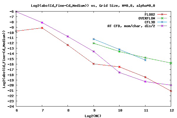
The figure below shows the log base two of the convergence rate of Cd for Mach=0.8 and α=0.00. Note that the 2nd order dissipation was set to 1.0 for Mach=0.8 due to difficulty converging the AT CFD residual for the Mach=0.80, α=1.25 case. The convergence rate for AT CFD when the 2nd order dissipation is set to 2.0 and 1.0 are very similar.
Shown below is the Cd data for M=0.8 and α=0.00. The AT CFD boundary condition is momentum and the surface boundary and characteristic at the far field boundary condition.
| NC | NC2 | FLO82-HCUSP | OVERFLOW-Central | AT CFD | CFL (AT CFD) | AT CFD, DIS2/2 | CFL (AT CFD, DIS2/2) |
| 32 | 1,024 | +0.011451356 | +3.148548e-02 | 16 | +2.762039e-02 | 16 | |
| 64 | 4,096 | +0.010264792 | +1.382376e-02 | 26 | +1.254787e-02 | 26 | |
| 128 | 16,384 | +0.008500758 | +9.245473e-03 | 34 | +9.007880e-03 | 34 | |
| 256 | 65,536 | +0.008312402 | +0.008734038 | +8.451336e-03 | 36 | +8.422317e-03 | 36 |
| 512 | 262,144 | +0.008328328 | +0.008493959 | +8.346057e-03 | 36 | +8.343248e-03 | 36 |
| 1,024 | 1,048,576 | +0.008338967 | +0.008412129 | +8.337990e-03 | 38 | +8.338199e-03 | 38 |
| 2,048 | 4,194,304 | +0.008341760 | +0.008376064 | +8.339357e-03 | 38 | +8.339724e-03 | 38 |
| 4,096 | 16,777,216 | +0.008342211 | +0.008358591 | +8.340418e-03 | 38 | +8.340694e-03 | 38 |
| ∞ | +0.008342298 | +0.008342171 | |||||
Boundary condition comparisons for AT CFD were not created for Mach=0.8 and α=0.00 due to a lack of resources.
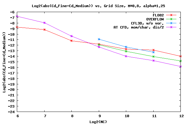
The figure below shows the log base two of the convergence rate of Cd for Mach=0.8 and α=1.25. Note that the 2nd order dissipation was set to 1.0 due to difficulty converging the AT CFD residual for this case. The convergence rate for AT CFD when the 2nd order dissipation is set to 2.0 and 1.0 are very similar for the data produced.
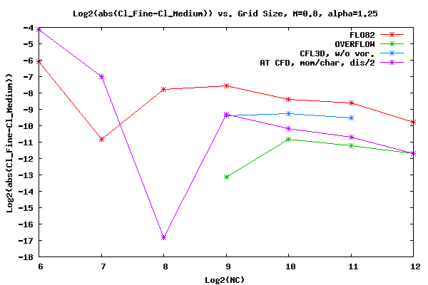
The figure below shows the log base two of the convergence rate of Cl for Mach=0.8 and α=1.25.
Shown below is the Cd data for M=0.8 and α=1.25. The AT CFD boundary condition is momentum and the surface boundary and characteristic at the far field boundary condition. The original 2nd order dissipation was set to 2.0 to match the default value in OVERFLOW. Unfortunately when the grid size reached 2048x2048 the CFL value for maximum convergence fell from 38 to 3. To run the 4096x4096 grid with a CFL value of 3 was impractical. Therefore, another set of runs was made using half the dissipative value, i.e. 1.0.
| NC | NC2 | FLO82-HCUSP | OVERFLOW-Central | AT CFD | CFL (AT CFD) | AT CFD, DIS2/2 | CFL (AT CFD, DIS2/2) |
| 32 | 1,024 | +0.027861593 | +0.03978770 | 16 | +0.03683203 | 16 | |
| 64 | 4,096 | +0.025487792 | +0.02882407 | 27 | +0.02760906 | 27 | |
| 128 | 16,384 | +0.023786371 | +0.02392013 | 36 | +0.02356254 | 36 | |
| 256 | 65,536 | +0.023357651 | +0.022964252 | +0.02288451 | 36 | +0.02278761 | 36 |
| 512 | 262,144 | +0.023084749 | +0.022706732 | +0.02262983 | 36 | +0.02259296 | 36 |
| 1,024 | 1,048,576 | +0.022934404 | +0.022593342 | +0.02254903 | 38 | +0.02253109 | 38 |
| 2,048 | 4,194,304 | +0.022799839 | +0.022534646 | +0.02250409 | 3 | +0.02249613 | 38 |
| 4,096 | 16,777,216 | +0.022737860 | +0.022500576 | +0.02247902 | 38 | ||
| ∞ | +0.022684938 | +0.022453440 | |||||
Shown below is the Cl data for M=0.8 and α=1.25.
| NC | FLO82-HCUSP | OVERFLOW-Central | AT CFD | AT CFD, DIS2/2 |
| 32 | +0.387842746 | +0.2752061 | +0.2910801 | |
| 64 | +0.372921380 | +0.3487919 | +0.3480884 | |
| 128 | +0.373469550 | +0.3578686 | +0.3557860 | |
| 256 | +0.368980205 | +0.353909135 | +0.3569911 | +0.3557945 |
| 512 | +0.363747900 | +0.353798330 | +0.3547914 | +0.3541939 |
| 1,024 | +0.360812844 | +0.353241712 | +0.3536338 | +0.3533173 |
| 2,048 | +0.358281928 | +0.352827907 | +0.3528566 | +0.3527142 |
| 4,096 | +0.357142338 | +0.352522552 | +0.3524159 | |
| ∞ | +0.356208937 | +0.351662793 | ||
Shown below is the Cm data for M=0.8 and α=1.25.
| NC | FLO82-HCUSP | OVERFLOW-Central | AT CFD | AT CFD, DIS2/2 |
| 32 | -0.042947499 | -0.03474209 | -0.03454162 | |
| 64 | -0.043584427 | -0.04185574 | -0.04038956 | |
| 128 | -0.043873739 | -0.04059599 | -0.03976616 | |
| 256 | -0.042552941 | -0.038987812 | -0.03959217 | -0.03922368 |
| 512 | -0.041002228 | -0.038656831 | -0.03881174 | -0.03864736 |
| 1,024 | -0.040136414 | -0.038402691 | -0.03845352 | -0.03837098 |
| 2,048 | -0.039388829 | -0.038251571 | -0.03822933 | -0.03819371 |
| 4,096 | -0.039051466 | -0.038150471 | -0.03810737 | |
| ∞ | -0.038774022 | -0.037946129 | ||
Boundary condition comparisons for AT CFD were not created for Mach=0.8 and α=1.25 due to a lack of resources.
References
1. ftp://cmb24.larc.nasa.gov/outgoing/Vassberg_2D_NACA00122. Vassberg, J. C., and Jameson, A., "In Pursuit of Grid Convergence, Part I: Two-Dimensional Euler Solutions," AIAA.2009-4114, June 2009.
3. Nichols, R. H., and Buning P. G., "User's Manual for OVERFLOW 2.1, Version 2.1t Aug 2008," Aug 2008.