Hegedus Aerodynamics
Lift on a 2D Series of Flat Plates
The following example describes the RANS CFD results for a series of 2D flat plates. The plates were created by splitting a 2D cylinder in half and inserting sections of various lengths between the cylinder halfs. The plate thickness, and thus cylinder diameter, is based on the approximate trailing edge thickness of a NACA 0012 airfoil. The freestream is at Mach 0.1 and the angle of attack is 1 degree. The Reynolds number is based on a value of 3e6 for the original NACA 0012 chord length. The overall case objective is to try to understand the Kutta condition, one of the assumptions required for the generation of lift for an airfoil, a little more.
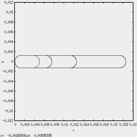
The plate thickness, non-dimensionalized by the NACA 0012 chord, is equal to 0.00252. Therefore, the Reynolds number based on the diameter is 7560.
Ten inserts were added. The lengths, non-dimensionalized by the NACA 0012 chord, were 0.0025, 0.005, 0.01, 0.02, 0.04, 0.08, 0.16 0.32, 0.64, and 0.99748
The first four geometries appear as follows.
For the CFD runs, the Spalart-Allmaras (SA) turbulence model was used. The number of points around the leading edge semi circle was 301 and the trailing edge semi-circle had the same amount. The number of points along the length of each insert were respectively: 101, 201, 201, 301, 401, 601, 801, 1001, 1001, and 1001. The number of points towards the outer boundary was 401 for all cases. The outer boundary was 150 NACA 0012 chords away from the surface. The first off body grid spacing was 2.4e-6 and represents a y+ of a little less than one based on the plate thickness. The code, Aero Troll CFD, is a 2nd order spatial discretized central difference method with artificial dissipation.
The following table shows the results. The reference length for cl is the chord of each geometry. For example, the reference chord for the first insert, 0.0025, was 0.00502. The cl was calculated with the pressure only, skin friction is not included. All results are fully converged.
| Insert Length | cl | Max Mach |
| 0.00250 | 0.091964 | 0.155 |
| 0.00500 | 0.102742 | 0.154 |
| 0.01000 | 0.108749 | 0.154 |
| 0.02000 | 0.111401 | 0.154 |
| 0.04000 | 0.111867 | 0.155 |
| 0.08000 | 0.111353 | 0.159 |
| 0.16000 | 0.110546 | 0.162 |
| 0.32000 | 0.109828 | 0.165 |
| 0.64000 | 0.109356 | 0.164 |
| 0.99748 | 0.109173 | 0.162 |
The theoretical lift (i.e. 2*pi*1 degree) for an airfoil is 0.10966.
The following plot shows the results.
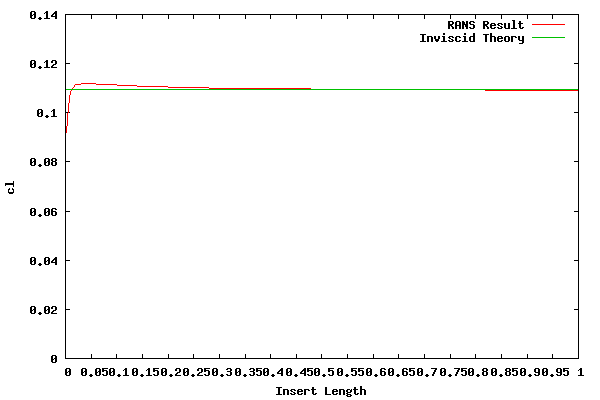
The above result showing the cl quickly reaching the theoretical value is somewhat surprising. Therefore, I'm skeptical the result accurately represents real world physics for the shortest plates.
The following plots show the cp distribution for each case.
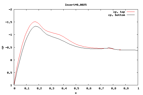
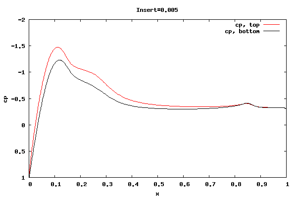
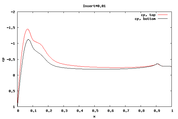
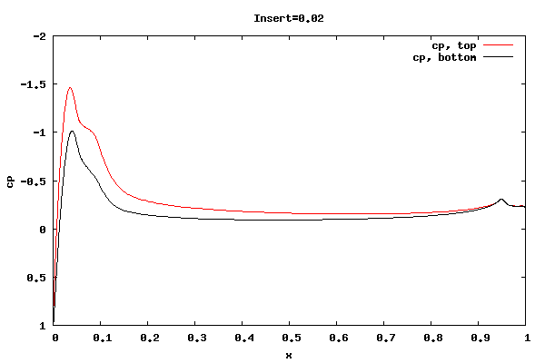
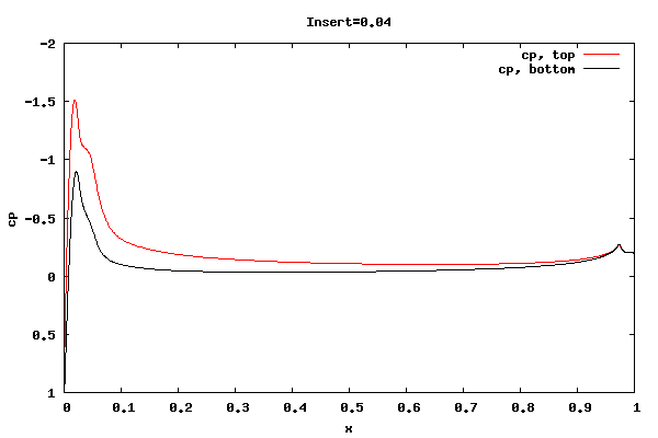
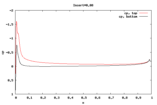

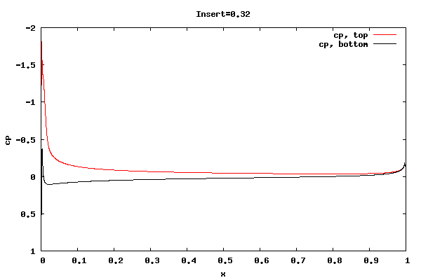
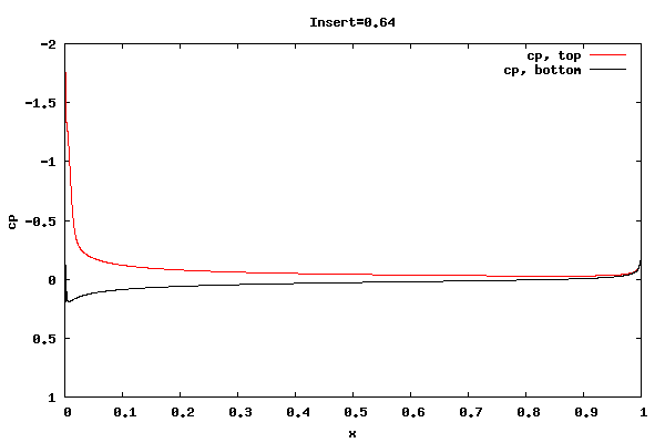

From the plots above it can be seen that the cp at the trailing edge is equal top and bottom indicating that the flow is leaving at the centerline of trailing edge rather than a point off the centerline. Therefore, the lift curve slope will be close to 2pi. Also, the pressure distribution at the leading edge indicates the presence of a separation bubble.
Whether the flow leaving at the centerline is an accurate physical description for the shorter rounded trailing edge geometries is unknown. I'm surmising the net vorticity in the separation bubble at the trailing edge is rotating counter clockwise, thus causing the rear stagnation point to move downward and create symmetric flow about the centerline. It could be that a true unsteady trailing edge separation bubble would not allow for it, thus reducing the lift.
The table below shows the lift and drag results for a series of runs done on the 0.005 insert case. The intent of the runs is to transition to a low artificial dissipation Euler run to witness how the results behave. As can be seen, even the low artificial dissipation Euler run has a substantial amount of lift. This is probably due to low order spatial discretization (1). Therefore, to reduce the error due to low order discretization and artificial dissipation, a high order code needs to be employeed to perform further studies.
| 0.005 Case | Slip | κ(4) | cl | cd | Max Mach |
| RANS | N | 0.04 | 0.102742 | 0.118787 | 0.154 |
| RANS | Y | 0.04 | 0.051508 | 0.000916 | 0.169 |
| Laminar | Y | 0.04 | 0.052769 | 0.000774 | 0.169 |
| Euler | Y | 0.04 | 0.064271 | 0.000375 | 0.171 |
| Euler | Y | 0.02 | 0.063937 | 0.000275 | 0.171 |
| Euler | Y | 0.01 | 0.063218 | 0.000212 | 0.171 |
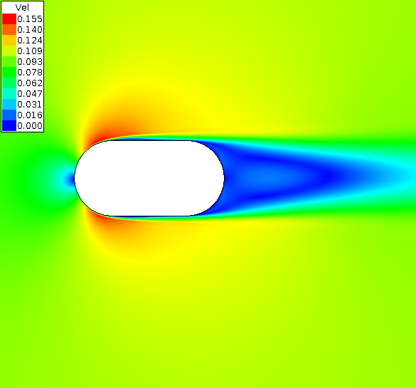
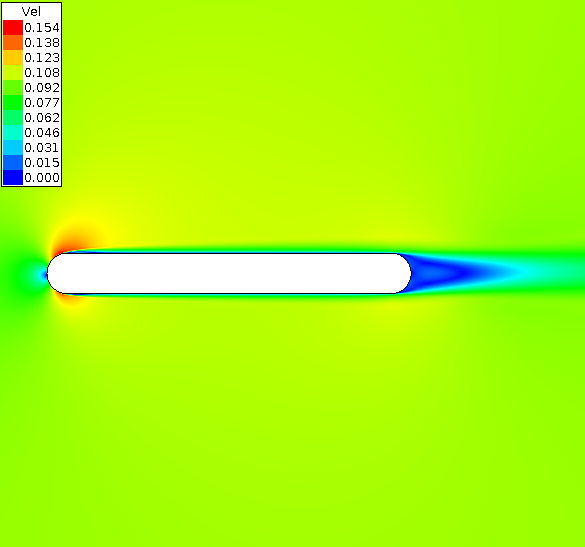
The following two plots show the velocity contours for the 0.0025 and 0.0200 RANS insert cases.
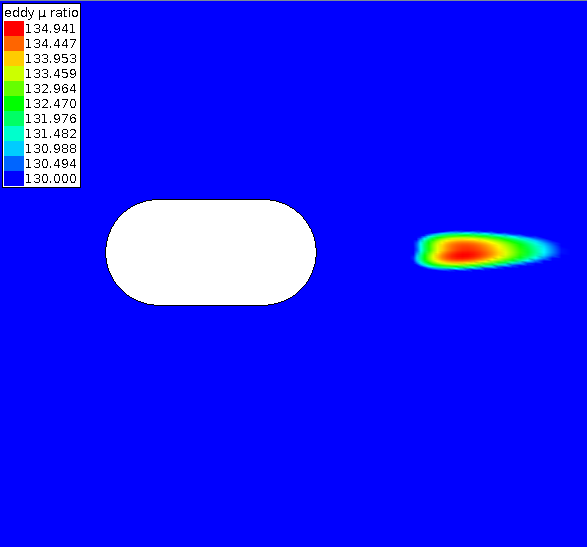
To get an idea of the amount of vorticity in the wake, the next plot shows the eddy viscosity for the shortest insert case. The contour plot range has been limited to help demonstrate that the eddy viscosity is not symmetric about the centerline. It can also be seen that more eddy viscosity is below the centerline indicating that the counter clockwise vortex below the centerline may have a larger magnitude than the clockwise vortex above the centerline. Therefore, the net vortex may be counter clockwise and pushing the stagnation point down.
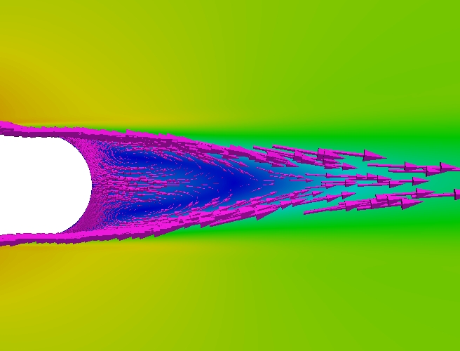
The next plot shows the velocity contour plot with arrows scaled based on the velocity magnitude for the wake region of the 0.0025 RANS insert case.
When all is said and done, I now have more questions about the "Kutta" condition on such a geometry than I began with.
References
1) Pulliam, T.H., "A Computational Challenge : Euler Solution for Ellipses," AIAA J., Vol. 28,No. 10, Oct. 1990.