Hegedus Aerodynamics

Separation From a Cone Cylinder Shoulder

The AT CFD results shown below for a pair of blunt cone-body shapes illustrate how two completely different solutions can be found depending on whether a local time step (CFL) or constant time step is used. The results are axisymmetric and for a Reynolds number of 45.0e6 based on the diameter. The Mach number is 0.9 and the angle of attack is 0.

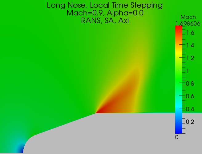
The first case I ran was for a blunt nose I call the long nose. For this case I marched the solution with a local time step (CFL) value of 5.0. This is standard procedure for obtaining steady state results since it converges the solution faster than a constant time step. The Mach number plot is shown below. The result was converged to machine zero (double precision).

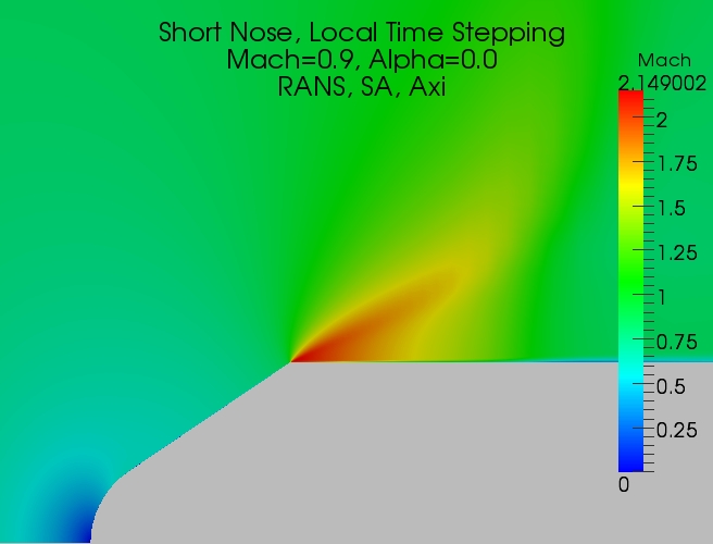
Next, I changed the angle of the nose cone by shortening the nose. The nose length is approximately 40% shorter than the nose length for the previous long nose example. The problem was converged with the same local time stepping approach used above. The Mach number plot for the short nose geometry with local time stepping is shown below and is qualitatively similar to the first. The result was converged to machine zero (double precision).

This is were the fun begins. The key to the fun is that I used a local time stepping method. With the local time stepping approach each grid cell is marched by a local time step which is a function of the grid cell size. The bigger the cell, the larger the time step. This is non physical.

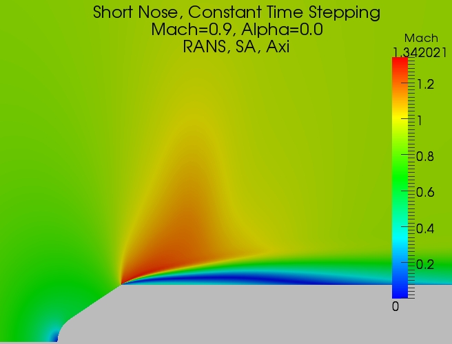
After seeing the result above, I was skeptical of the solution so I re-ran the case with a constant time step. Unfortunately, this takes more CPU time since the time step is constrained by the smallest cell size. These are the cells next to the body which are required to have a very small height to properly capture the boundary layer. The solution took about 20 times longer than the local time stepping approach.

The short nose geometry with constant time step result is shown below. The result was converged to machine zero (double precision). A separation bubble now exists. Also notice that something which looks like a shock is riding on top of the bubble. However, this is not a shock. The separation bubble adapts so that the flow can slow down without one. I do not know of a case in the real world, outside of the lab, where this happens. However, I've been told that this phenomenon can be reproduced in the lab.

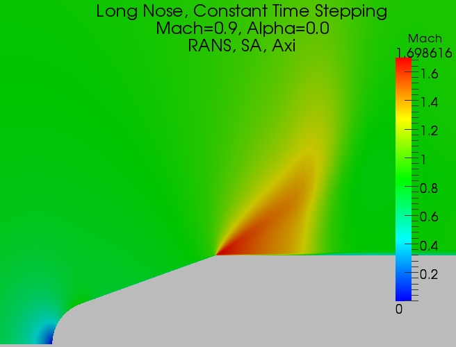
The final image, shown below, is the long nose geometry re-run with a constant time step. Notice it is very close to the result obtained with the local time stepping approach. Any difference is a result of the fact that I did not converge it all the way.